Easy methods to Use TODAY() to Spotlight Quick-Approaching Dates in an Excel Sheet

Products You May Like

Use Microsoft Excel’s TODAY() operate in easy expressions to spotlight the present date and previous and future dates.

Many functions observe dates for plenty of completely different causes. You may observe due dates, supply dates, appointments and so forth. Relying how you utilize these dates, you may wish to spotlight particular dates as they strategy the present date in Microsoft Excel. Equally, you may wish to spotlight future dates.

Utilizing the TODAY() operate and some conditional highlighting guidelines, you’ll by no means get caught unaware.

Leap to:

Spotlight right this moment in Microsoft Excel

When you in all probability gained’t wish to wait till a due date to begin a venture, highlighting the present date may also help warn you when timing is crucial. Fortuitously, Excel’s TODAY() operate all the time equals the present date, so that you don’t should replace the rule and even embody an enter worth.

SEE: Discover these 87 Excel tips every user should master.

Let’s add a conditional format that all the time highlights the present date:

1. Choose the cells or rows you wish to spotlight. On this case, choose B3:E12 — the information vary.
2. Click on the Residence tab, after which, click on Conditional Formatting within the Kinds group and select Spotlight Cells Guidelines.
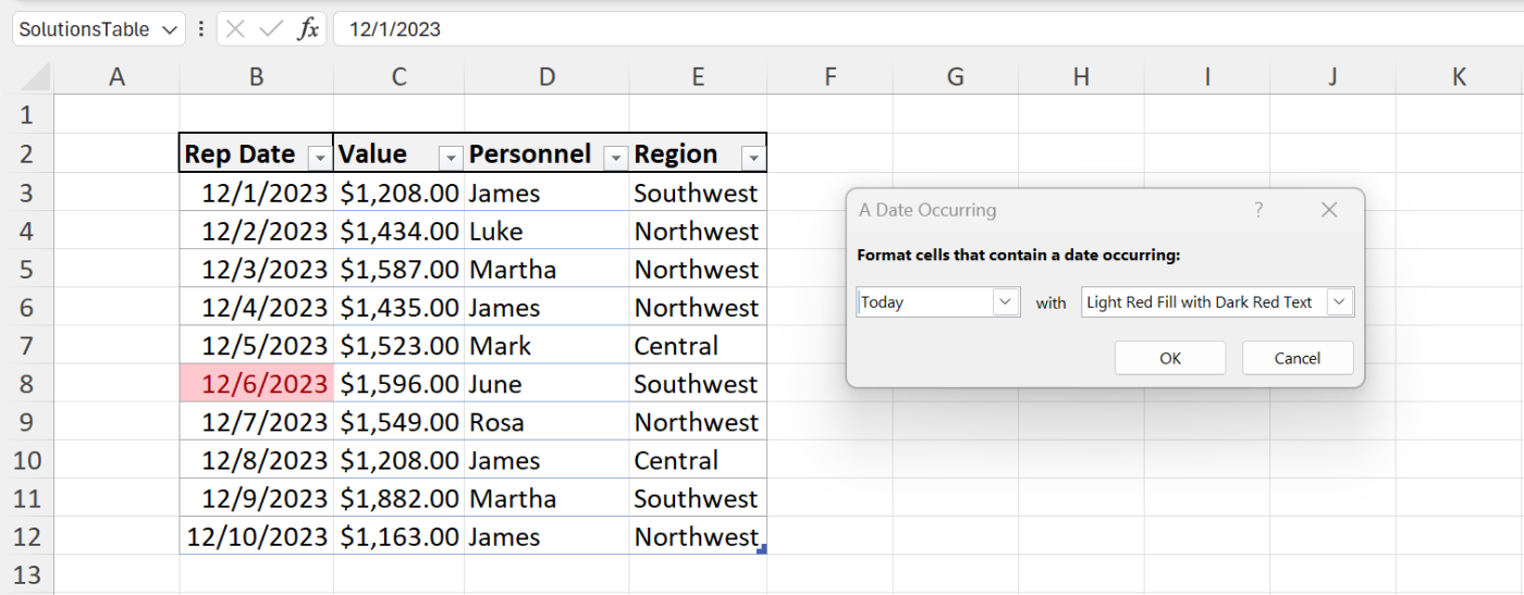
3. Select A Date Occurring.
4. Within the ensuing dialog, select As we speak from the primary dropdown, after which, select Gentle Crimson Fill from the second (Determine A). As you possibly can see, the present date is December 6.

Determine A

5. Click on OK.

This technique is the simplest method to shortly apply a conditional format to spotlight the present date, however it’s a bit restricted. First, you’ve just a few format mixtures accessible. Second, it doesn’t spotlight all the row — solely the cell containing the date. This rule is ready to detect dates within the chosen vary and apply the format solely to these cells. So, it doesn’t matter the place the date column is in relation to the chosen vary.

SEE: Try these ways to suppress 0 in Excel.

Spotlight yesterday in Microsoft Excel

There are built-in guidelines for yesterday and tomorrow, however let’s enter a rule as an alternative, so that you’ll know the way to take action when there isn’t an satisfactory built-in rule. Let’s begin with yesterday:

1. Choose the information vary B3:E12.
2. Click on the Residence tab. Then, click on Conditional Formatting within the Kinds group, and select New Rule.
3. Within the ensuing dialog, choose the Use a System to Decide Which Cells To Format possibility within the prime pane.
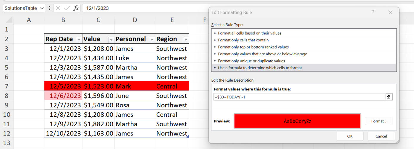
4. Within the backside pane, enter the expression =$B3=TODAY()-1. The straightforward expression TODAY()-1 subtracts one from the present date. That’s the identical factor as yesterday.
5. Click on Format.
6. Click on the Fill tab, select crimson and click on OK. Determine B exhibits the rule and the format.

Determine B

7. Click on OK to use the format.

As you possibly can see in Determine B, the rule highlights all the report when the date in column B is yesterday. Discover that the rule has an absolute column reference ($B). In the event you omit the greenback signal, Excel applies the spotlight to the cell as an alternative of all the row. The reference to row 3 isn’t absolute, so the rule can consider all the rows within the chosen vary.

SEE: Right here’s find out how to parse data in Microsoft Excel.

Spotlight tomorrow in Microsoft Excel

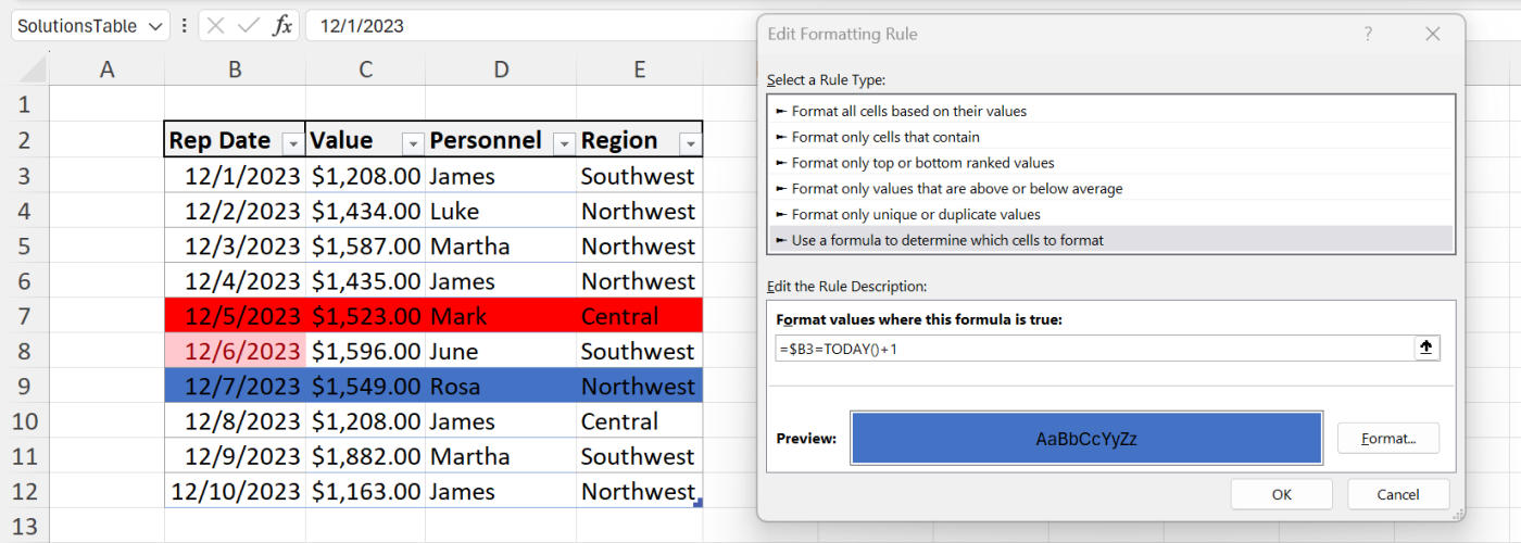
To focus on tomorrow, repeat the above steps, however enter the rule =$B3=TODAY()+1, as proven in Determine C. Click on Format, and select any shade, however I selected medium blue. Click on OK (twice) to use the format, which highlights all the row when the date in column B is tomorrow. Once more, absolutely the and relative referencing is essential.

Determine C

All three guidelines are easy to implement, however they’re restricted to right this moment, yesterday and tomorrow. What if you wish to spotlight different each day increments past these three?

Spotlight previous dates in Microsoft Excel

There could come a time while you’ll need a bit extra flexibility when highlighting essential dates. For example, you may wish to spotlight dates which might be every week forward or every week previous. When that is the case, I like to recommend utilizing an enter cell the place you possibly can specify the variety of days. By referencing the enter cell within the components, the spotlight will replace mechanically relying in your wants on the time.

Utilizing Determine D as a information, format two enter cells: days previously and days into the long run. Accordingly, we’ll reference C1 previously rule and C2 sooner or later.

Determine D

First, let’s enter the rule for the previous:

1. Choose the information vary B5:E14. Discover that I’ve up to date the vary rows as a result of I inserted rows for the enter cells.
2. Click on the Residence tab. Then, click on Conditional Formatting within the Kinds group, and select New Rule.
3. Within the ensuing dialog, choose the Use a System to Decide Which Cells To Format possibility within the prime pane.
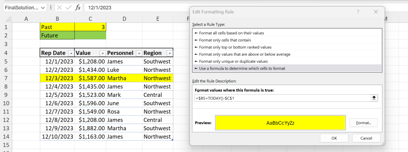
4. Within the backside pane, enter the expression =$B5=TODAY()-$C$1.
5. Click on Format.
6. Click on the Fill tab, select yellow and click on OK. Determine E exhibits the rule and the format.

Determine E

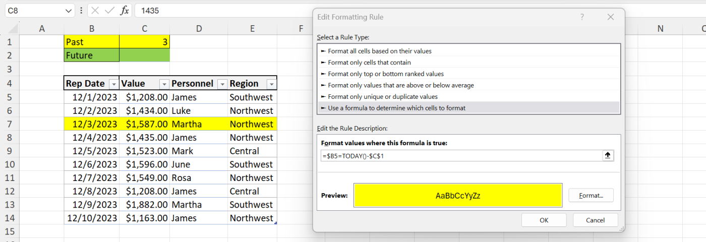
7. Click on OK to use the format.

Determine E exhibits the results of coming into 3 in C. As soon as once more, absolutely the handle, $C$1 is essential. In the event you depart this relative, the spotlight gained’t work as anticipated. When C1 is empty or incorporates 0, this rule highlights the present day.

SEE: Uncover find out how to adjust text to fit in Excel cells.

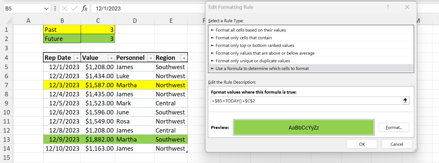
Spotlight future dates in Microsoft Excel

Repeat the steps above to use a spotlight for the long run. Besides in step 4, enter the expression =$B5=TODAY()+$C$2, and select inexperienced. Determine F exhibits the ensuing sheet after coming into the worth 3 into C2.

Determine F

With the enter cells and guidelines in place, be at liberty to alter the values in C1 and C2. If the worth is just too far into the previous or into the long run for the prevailing dates, Excel gained’t apply the spotlight. Go forward now and alter these dates to see how each guidelines work.

Useful hints

When making use of conditional codecs, the place of the rule is essential. The final guidelines you enter will take priority as a result of they’re the primary Excel evaluates. When a number of guidelines are in play, Excel won’t apply them within the order you anticipate.

To alter this, open the principles utilizing Handle Guidelines on the Conditional Formatting dropdown and transfer the principles accordingly. Yet one more factor that you just may contemplate. Use the fill shade of C1 and C2 to match the spotlight fill shade within the rule, as proven in Figures E and F. Doing so will provide a visible clue for the customers, so that they don’t have to recollect what these two colours imply.