Products You May Like
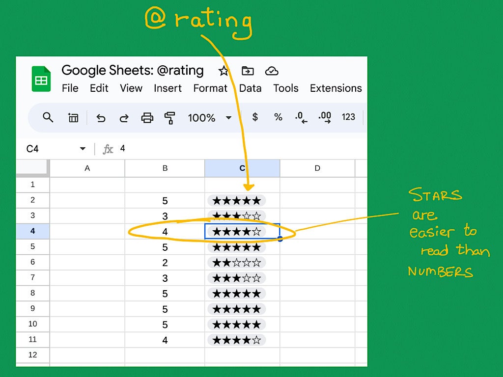
Sort @ranking so as to add a wise chip in Google Sheets on the net for a viewer-friendly solution to show zero-to-five star scores.
Google Sheets lets you enter star ratings in cells with a wise chip. Since many individuals discover stars simpler to distinguish at a look than an inventory of numbers, this function could also be helpful wherever you wish to charge merchandise, options, media, apps, locations or companies. The function gives the identical kind of 5-star format utilized in Android and Apple app shops and at Amazon, Uber and Yelp.
You could format cells for star scores in Google Sheets on the net. As soon as formatted, you might choose and enter a ranking both in Google Sheets on the net or within the Google Sheets cell apps on Apple or Android units.
Bounce to:
Tips on how to format a cell for stars in Google Sheets
Working with stars in a Google Sheet is a two-part course of. First, you configure a cell to indicate stars, and then you definitely or your collaborators can enter a star ranking. To format a cell for scores:
- Open a Google Sheet in an internet browser.
- Place your cursor in a Google Sheet cell.
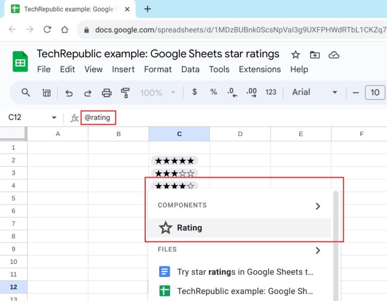
- Sort @ranking and press return or enter to pick the star ranking part from the good chip menu (Determine A). The newly formatted cell defaults to a numerical worth of zero and shows no stars.
Determine A
Tips on how to enter a star ranking in Google Sheets
As soon as a cell has been formatted to show a star ranking, you might enter the ranking both on the net or in Google Sheets on a cell system.
To enter stars whereas in an internet browser, corresponding to Google Chrome:
- Click on or faucet on the cell formatted for stars.
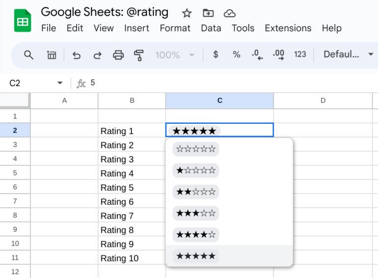
- From the six menu choices that show, choose wherever from 0 to five stars with a click on or faucet (Determine B).
Determine B
To enter stars within the Google Sheets cell app on Android, iPhone or iPad:
- Double faucet on a cell formatted for stars.
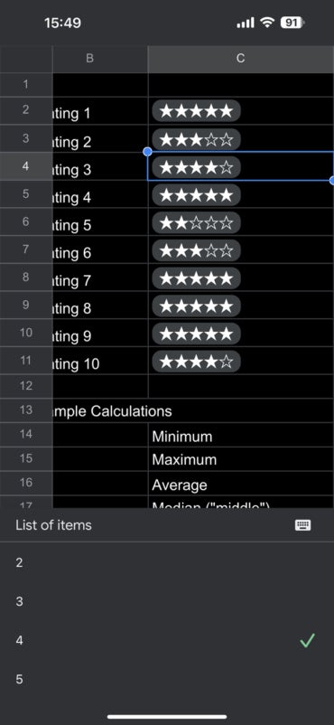
- Choose the variety of stars (i.e., 0 to five) you wish to enter from the listing that shows. You could must scroll down the listing a bit to faucet on the upper numbers (i.e., 4 and 5) (Determine C).
Determine C
Tips on how to use just a few formulation to judge star scores
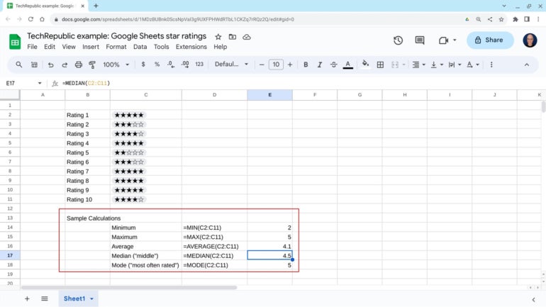
Scores in Google Sheets are mirrored because the numbers zero to 5, which implies you might receive values from every star ranking cell. The next formulation may also help you consider a spread of star scores in Google Sheets (Determine D).
Determine D
What are the bottom and highest scores?
The Min and Max formulation return the bottom and highest numbers from a set, respectively. For instance:
=Min(C2:C11)
=Max(C2:C11)
The distinction between the Min and Max signifies the total vary of individuals’s scores. For instance, a Min of three and a Max of 4 signifies settlement on a mid-range rating from responders, in comparison with a Min of 1 and a Max of 5, which alerts a wider vary of scores.
What’s the common ranking?
The typical of a set of stars will probably be someplace between 0 and 5, and might point out the general consensus throughout all scores. When evaluating two scores, the upper common typically displays general greater scores. To calculate the typical, the system provides all scores, then divides the overall by the variety of scores acquired. For instance:
=Common(C2:C11)
What’s the center ranking?
The median is the worth that separates a set in half, with half of the scores above the median and half of the scores under it. In distinction to the typical, which may be affected by just a few extraordinarily excessive or low scores, you would possibly consider the median as reliably reflecting the center of a set. To acquire the median, use a system corresponding to:
=Median(C1:C11)
What ranking was most supplied?
Mode returns the ranking most incessantly present in a set. For instance, in a set of 10 scores, if 4 of these are two stars, three are 4 stars, and three are 5 stars, the mode can be two stars. For instance:
=Mode(C2:C11)
Not like the above formulation, which can all the time return a outcome, Mode may not. For instance, in a set of 10 scores, if two individuals every rated gadgets one, two, three, 4 and 5 stars, there can be no mode. Since every of the attainable scores would have acquired two outcomes, there can be no single ranking that acquired probably the most. Equally, if star scores are break up between two numbers (e.g., 5 individuals rated an merchandise as 4 stars, and 5 individuals rated it as 5 stars), once more, there can be no mode.
Point out or message me on Mastodon (@awolber) to let me understand how you employ star scores and associated calculations in Google Sheets.